
The year was 1994, a retired professor named Leo Breiman published a small technical report called the “Bagging Predictors”. This turned out to be the most influential idea in modern machine learning. I always have a lingering thought that most of the machine learning and deep neural networks theory has been around for a very long time, and wonder that students should look at the past, to try and understand the concepts better instead of chasing the latest and the greatest.
Let’s start straight with an analogy. Imagine you’re faced with a critical decision and seek advice from experts. Instead of relying on the suggestion of one master expert you decide to consult many good enough experts. Each expert provides a unique perspective, that guides you to make the best choice. The Random Forest algorithm operates similarly. It assembles many decision trees hence the term “Forest”, by randomly choosing data, hence the term “Random” and averages out the prediction from all the learned trees.
Here is the procedure that Breiman proposed:
- Bootstrap replicates of your learning set: Randomly choose a subset of rows from your data.
- Train a model and save it.
- Return to the first step many times.
- This gives many saved models, the predictions of which are averaged for the final prediction.
The above procedure is called bagging. It is based on an insight that although each of the models will make errors, they will be different and not correlated to each other. I will discuss the mathematics of this in another blog and it is quite elegant.
Breiman later went on to demonstrate that along with randomly choosing rows of the data, if we also randomly select columns of the data at each split of the decision tree, the accuracy can be improved further. This algorithm is the famous “Random Forest”.
Let us look at what is a decision tree. Since we are talking about forests.
Decision Tree
Decision Trees (DTs) are a non-parametric supervised learning method used for classification and regression. The goal is to create a model that predicts the value of a target variable by learning simple decision rules inferred from the data features. A tree can be seen as a piecewise constant approximation.
https://scikit-learn.org/stable/modules/tree.html
Hold On! I will be simplifying the above statement before we break out the pitchforks. Alright, Let’s go:
A decision tree is a way of making choices based on some information. For example, Let’s take the data below consisting of 100 entries. Our task is to predict the income of a person based on the age and the amount spent by the person.

Below is what the decision tree for the same looks like:
This has been programmatically generated using the sklearn library. Additional Annotations are done by me.
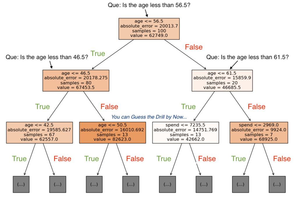
Basically decision tree is just a series of questions asked at each split, at the first level called the root node the question asked is “Whether the age of the person is less than 56.5 or greater?”.
The data is split two ways one way contains where the condition is TRUE while the other way contains data where the condition is FALSE.
Similarly, data is further split based on different questions asked at each node until a stopping criterion is met which is usually the max depth of the tree. Now Imagine a tree that is allowed to split as many times as it likes. I urge the reader to pause and ponder on how this tree would come to fruition and why such a tree is not feasible.
The “samples” in each node is the number of training samples in that node which fulfills the splitting criterion. The “value” is the average value of the target based on the samples in the node, in our case the income field. The “absolute_error” is the average value predicted by the tree minus each of the entries divided by the total entries. This is the criterion that we would like to minimize.
Some words that you may not know are:
- Non-parametric: This means that the decision tree does not tie weights to the columns of the data. It can adapt to any kind of data and find the best way to split it into branches.
- Supervised learning: This means that the decision tree learns from some examples or data that have the correct answers or labels. In our example, we had 100 entries with the target income which we used to fit the data.
- Target variable: This is the thing that you want to predict or classify using the decision tree. In our example, the income is the target variable.
- Data features: These are the things that describe the data or the information that you have. The “age” and “spend” columns are the data features in our case.
- Decision rules: These are the questions or the criteria that the decision tree uses to split the data into branches. These are the questions asked at each split based on a column of the dataset. The annotated questions in the diagram.
- Piecewise constant approximation: A very heavy word IMO! Let’s look at a simple analogy.
Imagine you have a drawing of a mountain, like this:
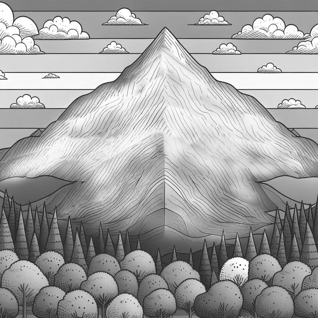
The mountain has different heights at different places, right? But what if you want to make a simpler drawing of the mountain, using only a few colors and lines? How would you do that?
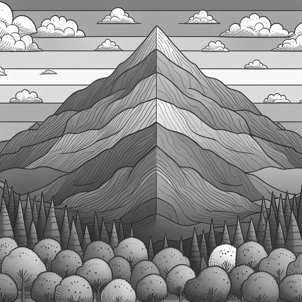
One way is to use piecewise constant approximation. This means you divide the mountain into small pieces, and for each piece, you choose a color that is close to the average height of the mountain in that piece. Then you fill the piece with that color and draw a line at the top of the piece. For example, you can divide the mountain like this:
And then you can choose these colors for each piece:
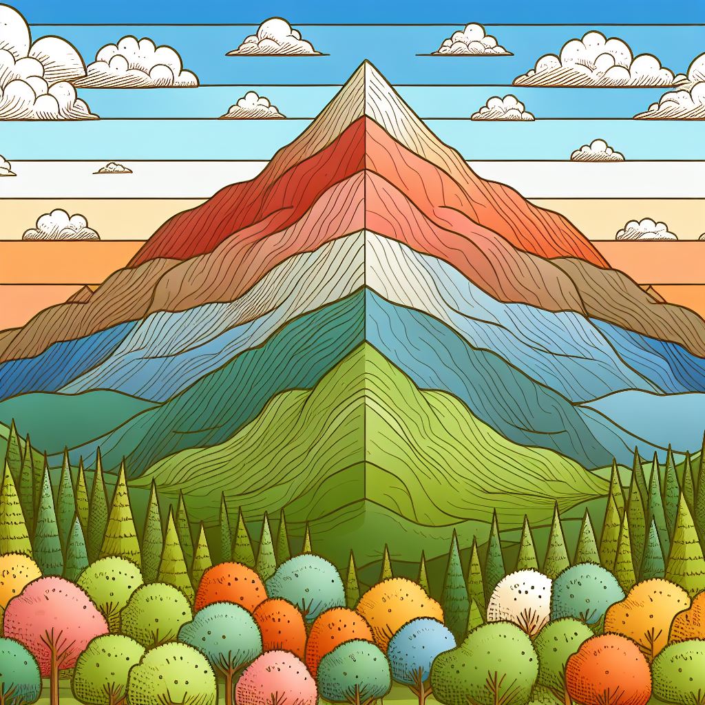
Now you have a simpler drawing of the mountain, using some colors and lines. This is called piecewise constant approximation because you approximate the mountain with pieces that have constant (or the same) colors and heights.
I had the last image generated by Dall-E 3. I photoshopped the other two. Mad Photoshop skills IMO!
Below is a decision tree fitted to a sine curve at two different depths 2 and 5. The tree uses if-then-else statements which we discussed above.
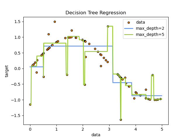
The function has steps in it rather than being continuous. The tree approximates a constant value for a given range of input values.
The tree with max_depth of 2 seems rather simple, which given room for more depth can fit the data better. This is a case of underfitting.
On the contrary, the tree of max_depth of 5 seems more complex and has even fit the outliers perfectly well. This seems good from the perspective of training data but the model will fail when extrapolating to new unseen data. This is a case of overfitting.
In machine learning, we always strive for the optimal value in between. Not too over-fit, not too under-fit.
Conclusion
The Random Forest Algorithm is just many of these decision trees combined, built using random subsets and random features from our training data. We have seen how it builds on the ideas of bagging, decision trees, and piecewise constant approximation to create a robust and accurate model that can handle both classification and regression problems. Random Forest is one of the most popular and widely used algorithms in machine learning, and I hope this blog has helped you understand its inner workings better.
Thank you for reading and happy learning! 😊
While reading the bagging paper by Leo Breiman, I came across the mathematics of why bagging works which I would love to delve deeper into. Perhaps that can be a follow-up blog. Peace!!
References:
- scikit-learn developers. (2020). Decision trees. https://scikit-learn.org/stable/modules/tree.html
- Breiman, L. (1996). Bagging predictors. Machine Learning, 24, 123-140.
- Howard, J., & Gugger, S. (2020). Tabular Modeling Deep Dive. In Practical deep learning for coders (pp. 277-329). O’Reilly.

Leave a Reply