
Our very random universe we perceive is not so random after all. At least, that’s what the statisticians say and they have enough data to prove it. The central limit theorem(CLT) governs most of the processes of the universe, saying when you look at the bigger picture it is just the average of it all. Yes, that is it. The definition goes as follows:
As the size of a randomly drawn sample from a population increases, the distribution of the sample mean will converge towards a normal distribution, regardless of the underlying distribution of the population itself, under the following conditions:
Independent and identically distributed (i.i.d.) samples:
- Each observation within a sample must be independent of the others.
- All samples must be drawn from the same population distribution.
Finite variance:
- The population variance must be finite, meaning it cannot be infinite.
Alright let’s break it down with an analogy:
Imagine a giant bag filled with many many many marbles(say 10 million) of different weights, some weigh very heavy while some are light as a feather, also the proportion of the different weighing marbles varies too much. This bag represents the entire population you’re studying.
Suppose you take 30 marbles from the bag every time, weigh them, and plot them.
Independent and Identically Distributed (i.i.d.) Sampling:
- Independent: When you grab the marbles, you do it without peeking. Each marble you pick is independent of the others, meaning it doesn’t influence the next batch of 30 marbles. They are not arranged in a specific pattern. Also, you put the marbles back into the bag after weighing one batch. (Truly Independent Samples)
- Identically Distributed: You always draw from the same bag, ensuring that all samples represent the same overall population. You’re not switching to a different bag halfway through.
Finite Variance:
- The marbles in the bag aren’t all the same size or weight. Some are very heavy while others are light—that’s the variance. But there’s a limit to how much they can vary. You won’t find a marble as big as a basketball or as tiny as a grain of sand in this bag. The variation is reasonable and finite.
Now, let’s see the CLT in action:
Multiple Handfuls:
- You keep grabbing a batch of 30 marbles(random samples) from the bag, each time counting the average weight of the marbles in your hand.
Surprising Pattern:
- As you collect more and more handfuls, you notice something fascinating: The graph of all those average weights starts to form a bell-shaped curve, even if the marbles themselves have a very different distribution of weights!
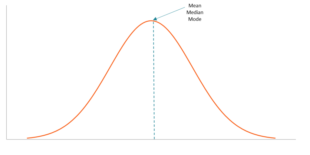
Fancy Name: Gaussian Distribution.
Now a burning question why a sample size of 30 and not greater or less than that.
Well sample size of more than 30 is perfectly acceptable you can take a million samples and weigh them. But the problem starts when you take a sample size of less than 30 samples. After years of applying this theorem, statisticians concluded that a sample size of more than 30 is appropriate. However, for some rare cases, sample size of less than 30 can be considered valid as well.
Law of large numbers:
Before we head further let’s look at another concept from probability theory called the law of large numbers. In simple terms, the theorem says that if you take the average of large enough samples, the average will approach the true average of the system.
Analogy alerts:
Imagine flipping a coin many times. You might get head or tails. As you repeat the experiment with more and more coin flips, the proportion of heads will tend closer and closer to 50%(Average of the system).
The graph would look something like this:
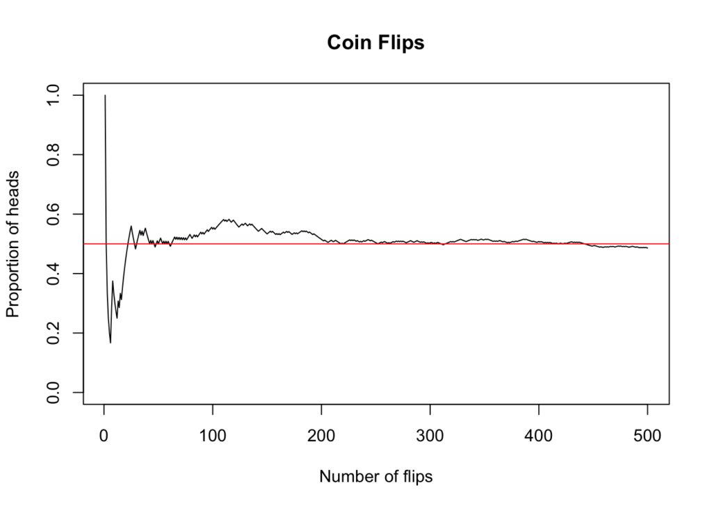
This theorem was proven by mathematician Jacob Bernoulli in 1713. This is the theorem that helps casinos make money in the long run. Next time you go to a casino make sure to buzz off and sleep as soon as you win, because sitting there is guaranteed(almost) to make you lose money.
Deep Learning and CLT:
Most of the neural networks today are trained using stochastic gradient descent(or a version of it) in a parametric fashion. However, their inner workings are still a black box. The Central Limit Theorem can take us closer to understanding the inner workings of a neural network.
Let’s look at where CLT might help:
- Weights and biases: Deep Learning Models rely on random initialization of the weights and biases. This is a very important step, not doing this correctly can lead to the network not converging. The central limit theorem guarantees(almost) that the randomly initialized parameters will follow a Gaussian distribution (Fancy word for the bell curve we saw above), smoothing out the impact of individual random values and promoting stable learning.
- SGD: The word stochastic in stochastic gradient descent means random. It can be deduced that showing random batches of the training data can lead to the network estimating the true mean of the entire population(”Test Set + Training Set” and beyond).
- Dropout: By randomly dropping out neurons during training, dropout introduces noise into the learning process and helps mitigate overfitting. The CLT provides a theoretical basis for why this stochasticity can be beneficial, preventing overfitting by averaging out the influence of individual neurons.
- Ensemble Learning: Ensemble methods, like bagging and boosting, combine predictions from multiple models trained on different subsets of the data. The CLT contributes to the effectiveness of these methods by suggesting that averaging the predictions of individually noisy models leads to a more accurate and robust overall prediction.
The Central Limit Theorem can also help explain why the neural network converges in the first place, and also why we see(possibly) generalization to out-of-distribution data.
Here are some interesting works related to CLT and Deep Learning:
Mean Field Analysis of Neural Networks: A Central Limit Theorem(2018) by Justin et al.:
- They rigorously prove the central limit theorem applicable to neural network models with a single hidden layer. Warning: Only the Math Wizards may proceed with this.
The central limit theorem in terms of convolutions by Maxwell Peterson:
- Excellent blog on convolutions and central limit theorem. It has great visualizations as well. Highly recommend reading it.
Peace! See you at the next one!!
References:
Wikipedia:
- Central Limit Theorem. (2023, December 19). In Wikipedia. Retrieved January 7, 2024, from https://en.wikipedia.org/wiki/Central_limit_theorem
Investopedia:
- Central Limit Theorem (CLT). (n.d.). In Investopedia. Retrieved January 7, 2024, from https://www.investopedia.com/terms/c/central_limit_theorem.asp
And all the awesome papers mentioned in further reads.


Leave a Reply