Deep Learning Blog

Entropy is a concept that is often associated with mystery and intrigue. It is a measure of the randomness or disorder of a system and can be used to describe everything from the behavior of atoms and molecules to the flow of information in a communication system. The entropy meaning has many faces and one will get different answers based on whom you ask. The term was first introduced by German physicist Rudolf Clausius in 1850 and has since been applied in a variety of fields, including thermodynamics(second thermodynamic law), statistical physics, information theory, and more.

We will be discussing entropy in terms of machine learning and artificial intelligence. This word comes up a lot in literature and research papers. Many deep learning and traditional machine learning models work because we have the concept of entropy with us. Let’s try to simplify some of the mystery around this word and gain a better understanding. Before diving deep into entropy and getting dispersed(pun intended), we will need to understand the notion of expected value. Fancy word, simple meaning. Let’s go!

Expected value

Expected value is a concept that helps us understand the average or most likely outcome of a random situation. It is based on the idea of multiplying each possible outcome by its probability and then adding them up. Let’s take an analogy to understand the above statements better.

Picture a magical vending machine, which has two types of coins. It dispenses enchanted coins of gold and silver. The gold and silver coins have a property that when you touch them something happens in your bank account.

Our magical machine has its own way of determining which coin to produce:

• Probability of a golden coin: P(Golden)=0.8
• Probability of a silver coin: P(Silver)=0.2

Each coin has a corresponding “value”:

• Value of a golden coin: $10 (because gold is precious, right?)
• Value of a silver coin: -$5 (because of that mischievous spell causing minor inconveniences)

Let’s say we have drawn a coin 100 times from the vending machine with the above probability. The probability of a gold coin is 0.8 meaning 80 times out of 100 we expect a gold coin. The value associated with it is $10. Hence the total gain from gold coin will be 80 * $10 = $800.

Similarly, we expect to draw silver coins 20 times. The value is -$5, hence the total gain will be 20 * -5$ = -$100

The result will be $800 – $100 = $700. Note that we can divide the result by the number of trials(100) and we get an expected value of $700/100 = $7 on every draw. So, on average, every time you use the enchanted coin machine, you can expect an outcome that’s worth $7.

This is the original formula for expected value:

E(X) = \sum x \cdot P(X = x)

Where x is the amount we gain or lose from a coin and p(X=x) is the probability of drawing the respective coins from the vending machine.

Pretty alien at first sight but trust me this is it. (Applicable to discrete random variables. The formula changes for other types of distribution. I highly recommend looking it up and making sense of it.). Now let’s address the elephant in the room “Entropy”

Entropy

Entropy, a concept rooted in thermodynamics, has found applications in various fields. In the context machine learning and data science, entropy provides a powerful measure that captures the degree of uncertainty, disorder, or surprise in a system.

Let’s take an example:

Suppose there is a butterfly guessing contest and someone has gathered lots of butterflies with two colours being blue and orange. There are three boxes of butterflies to pick from. The first box has a lot of blue butterflies and some orange butterflies:

The probability of picking a blue butterfly is very high from this box as there are more blue butterflies. It would be very surprising if someone picked up an orange butterfly from this box.

The second box has a large number of orange butterflies:

Similarly picking a blue butterfly from this box would be very surprising as well.

The third box has an equal number of orange and blue butterflies:

Picking a random butterfly from this box will surprise us equally no matter what the color of the butterfly is.

Think about it, Let’s say the proportion of blue butterflies in the first box is 90%, and the proportion of orange butterflies will be 10%(unless you live in a world where things max out at 200%). The surprise for picking an orange butterfly will be very high and hence it can be thought that the surprise is inversely proportional to the probability(0.1). The lower the probability of getting a thing the higher the surprise when we get it.

However, there is a problem by directly taking the inverse of probability as the surprise value. Suppose we have a box of butterflies filled only with blue butterflies. The odds of getting a blue butterfly will be 1 while that of an orange butterfly is 0. When we take the inverse of this:

\frac{1}{P(\text{Blue})} = \frac{1}{1} = 1

We do not want the surprise of getting a blue butterfly to be 1. It should be 0 we will always get a blue butterfly(Not surprising at all). Because of this we instead take the log of the inverse of probability as a measure of surprise. The above equation will evaluate to:

\log\left(\frac{1}{P(\text{Blue})}\right) = \log\left(\frac{1}{1}\right) = 0

In contrast, when we assess the surprise of getting an orange butterfly, we get the following equation:

\log\left(\frac{1}{P(\text{Orange})}\right) = \log\left(\frac{1}{0}\right) = \log(1) - \log(0) = \text{undefined}

This is what the graph of log(1/probability) looks like:

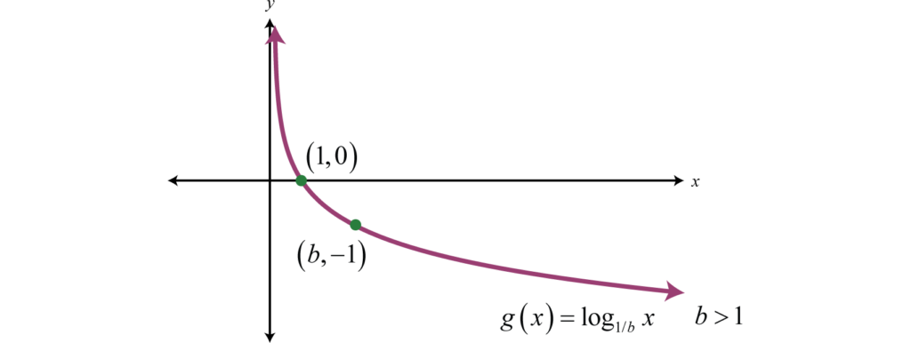
When the probability of getting a thing is 1 the surprise is 0. Similarly, If the probability of getting a thing is 0 we want our surprise to be undefined. Note: When calculating the surprise for two variables, in this case, the two types of butterflies, it is required to use the log base 2 to calculate the surprise.

Now Hold on bud! Aren’t we supposed to talk about entropy where did this surprise come from? Okay, we grab one of our boxes where we have a large number of blue butterflies and some orange butterflies. Suppose the probability of getting a blue butterfly is 0.75 and the probability of getting an orange butterfly is 0.25. First, we calculate the surprises for both the butterflies.

The surprise of getting a blue butterfly will be:

\log\left(\frac{1}{P(\text{Blue})}\right) = \log\left(\frac{1}{0.75}\right) \approx 0.29

Similarly, the surprise for getting an orange butterfly will be:

\log\left(\frac{1}{P(\text{Orange})}\right) = \log\left(\frac{1}{0.25}\right) \approx 1.39

Suppose we make 100 draws from the box and pick a butterfly. The surprise for getting blue is 0.29 while for an orange is 1.39. We want to calculate the total surprise for the 100 draws. Recall from the expected value part how can this be calculated.

(0.75 \times 100) \times 0.29 + (0.25 \times 100) \times 1.39 = 56.5

That will be the total surprise for the 100 draws. After dividing by 100 we get:

\frac{56.5}{100} \approx 0.57

0.57 is the expected surprise for a single draw from the box of butterflies. And this is “wait for it…..” the entropy of the system. Since we first multiply the equation with 100 and then divide it by 100 the calculation of entropy can be reduced down to:

(0.75 \times 0.29)  + (0.25 \times 1.39) \approx0.57

The above equation can be re-written with the fancy sigma notation:

\sum\nolimits x \cdot P(X=x)

Where x is the value of surprise for each of the butterflies and P(X=x) is the probability of seeing the butterfly. Plugging in the equation for surprise which we derived earlier our equation will turn out to be:

\sum\nolimits \log\left(\frac{1}{P(x)}\right) \cdot P(x)

Pretty amazing how we can complicate such an intuitive concept. Unfortunately, this is not the equation we are used to see out in the jungle.

The final equation will be as below:

\begin{align*}\sum\nolimits P(x) \cdot \log\left(\frac{1}{P(x)}\right) \\\sum\nolimits P(x) \cdot \left[\log(1) - \log(P(x))\right] \\\sum\nolimits P(x) \cdot \left[0 - \log(P(x))\right] \\\sum\nolimits -P(x) \cdot \log(P(x)) \\-\sum\nolimits P(x) \cdot \log(P(x))\end{align*}

This is the equation of entropy that Claude Shannon derived in 1948 while working at Bell Telephone Laboratories. Pretty Neat for an equation!

Some food for the brain:

• Can you calculate the entropy of the second box of butterflies where p(Orange) is 0.60 and p(Blue) is 0.40? What is the difference in surprise and why?
• How might an understanding of entropy influence data compression techniques?
• I cannot recommend enough this YouTube channel. One of the best out there to learn statistics. https://www.youtube.com/@statquest

References:

• Starmer, J. (Presenter). (, Month Day). Entropy (for data science) Clearly Explained!!! [Video]. YouTube. StatQuest with JoshStarmer. [https://www.youtube.com/watch?v=YtebGVx-Fxw&t=30s]